Tutorial: Fundamentals of deep learning

Administrative Information

Title	Tutorial: Fundamental of deep learning
Duration	180 min (60 min per tutorial)
Module	B
Lesson Type	Tutorial
Focus	Technical - Deep Learning
Topic	Forward and Backpropagation

Keywords

forward propagation,backpropagation,hyperparameter tuning,

Learning Goals

• student understands the concept of forward propagation
• student get view on how to derive backpropagation
• student can apply backpropagation
• student learns the way of tuning hyperparameters

Expected Preparation

Lesson materials

None.

Instructions for Teachers

This Learning Event consists of three sets of tutorials covering fundamental deep learning topics. This tutorial series consists of providing an overview of a forward pass, the derivation of backpropagation and the use of code to provide an overview for students on what each parameter does, and how it can affect learning and convergence of a neural network:

1. Forward propagation: Pen and paper examples, and python examples using Numpy (for fundamentals) and Keras showing a high level module (which uses Tensorflow 2.X).
2. Deriving and applying backpropagation: Pen and paper examples, and python examples using Numpy (for fundamentals) and Keras showing a high level module (which uses Tensorflow 2.X).
3. Hyperparameter tuning: Keras examples highlighting exemplar diagnostic plots based on the effects for changing specific hyperparameters (using a HCAIM example dataset Data sets for teaching ethical AI (Census Dataset).

Notes for delivery (as per lectures)

• Use of Sigmoid in the outer layer and MSE as the loss function.
  • With tine limitations, a singular approach/topology/problem context was selected. Typically, one would start with regression for a forward pass (with MSE as the loss function), and for deriving backpropagation (thus having a linear activation function in the output layer, where this reduces the complexity of the derivation of the backpropagation function), Then one would typically move to a binary classification function, with sigmoid in the output layer, and a binary cross-entropy loss function. With time constraints this set of lectures will use three different example hidden activation functions, but will use a regression problem context. To add the complexity of a sigmoid activation function in the output layer, the regression problem used in the two first lectures of this set, the problem example is based on a normalised target value (0-1 based on a percentage grade problem 0-100%), thus sigmoid is used as an activation function in the output layer. This approach allows students to easily migrate between regression and binary classification problems, by simply only changing the loss function if a binary classification problem, or if a non-normalised regression problem is being used, the student simply removes the outer layer activation function.
• Core components are the application of, using a high level library, in this case KERAS via the TensorFlow 2.X library.
  • Pen and paper are optional and only used to show the forward pass and backpropagation derivation and application (using the examples from the lecture slides).
  • Python code without use of high level libraries, is used to show how simple a neural net (using the examples from the lecture slides). This also allows for discussion on fast numerical/matrices multiplication and introduce why we use GPUs/TPUs as an optional element.
  • KERAS and TensorFlow 2.X are used and will be used for all future examples.

Tutorial 1 - Forward propagation

Teacher instructions

• This tutorial will introduce students to the fundamentals of forward propagation for an artificial neural network. This tutorial will consist of a forward pass using pen and paper, using Python with only the Numpy library (for matrices manipulation) and then using KERAS.. This will build upon the fundamental understanding of what activation functions apply to specific problem contexts and how the activation functions differ in computational complexity and the application from pen and paper, to code from scratch using Numpy and then using a high level module -> Keras.
• The students will be presented with three problems:
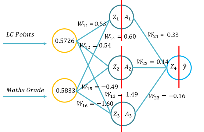
  • Problem 1: (Example 1 from the lecture -> Image on the RHS of this WIKI) and asked to conduct a forward pass using the following parameters (20 minutes to complete):
    • Sigmoid activation function for the hidden layer
    • Sigmoid activation function for the outer layer
    • MSE loss function
  • Problem 2: (Example 1 from the lecture), students will be asked (with guidance depending on the prior coding experience) to develop a neural network from scratch using only the Numpy module, and the weights and activation functions from problem 1 (which are the same as Example 1 from the lecture (20 minutes to complete).
  • Problem 3: (Example 1 from the lecture and using the same example but random weights), students will be asked (with guidance depending on the prior coding experience) to develop a neural network using the Tensorflow 2.X module with the inbuild Keras module, and the weights and activation functions from problem 1, and then using random weights (which are the same as Example 1 from the lecture: 20 minutes to complete).
• The subgoals for these three Problems, is to get students used to the structure and application of fundamental concepts (activation functions, topology and loss functions) for deep learning.

Time: 60 minutes

Outline/time schedule

Duration (Min)	Description
20	Problem 1: Pen and Paper implementation of a forward pass (example from the lecture)
20	Problem 2: Developing a neural network from scratch using Numpy (example from the lecture)
10	Problem 3: Developing a neural network from using Keras (example from the lecture with set weights and random weights)
10	Recap on the forward pass process

Tutorial 2 - Derivation and application of backpropagation

Teacher instructions

• This tutorial will introduce students to the fundamentals of the backpropagation learning algorithm for an artificial neural network. This tutorial will consist of the derivation of the the backpropagation algorithm using pen and paper, then the application of the backpropagation algorithm for three different hidden layer activation functions (Sigmoid, Tan H and ReLu), using Python with only the Numpy library (for matrices manipulation) and then using KERAS.. This will build upon the fundamental understanding varying activation functions when a neural network learns and how the activation functions differ in computational complexity and the application from pen and paper, to code from scratch using Numpy and then using a high level module -> Keras.
• Note: The topology is the same as Lecture 1/Tutorial 1, but the weights and inputs are different, you can of course use the same weights.
• The students will be presented with four problems (the first being optional or as additional material):
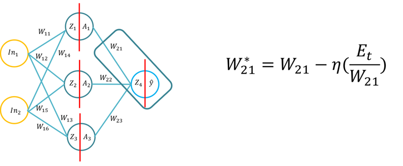
  • Problem 1: The derivation of the backpropagation algorithm (using the Sigmoid function for the inner and outer activation functions and MSE as the loss function), students will be asked to derive the backpropagation formula (20 minutes to complete).
  • Problem 2: Students will apply three activation functions for a single weight update (SGD backpropagation), using pen and paper for (20 Minutes):
    • Sigmoid (Hidden layer), Sigmoid (Outer Layer) and MSE
    • Tan H (Hidden layer), Sigmoid (Outer Layer) and MSE
    • ReLu (Hidden layer), Sigmoid (Outer Layer) and MSE
  • Problem 3: Students will be asked (with guidance depending on the prior coding experience) to develop a neural network from scratch using only the Numpy module, and the weights and activation functions where the option to select from any one hidden layer activation function is provided to update the weights using SGD (20 minutes to complete).
  • Problem 4: Students will be asked (with guidance depending on the prior coding experience) to develop a neural network using the Tensorflow 2.X module with the inbuild Keras module, and the weights and activation functions, and then using random weights to complete one or several weight updates. Please not as Keras uses a slight different MSE loss, the loss reduces quicker in the Keras example.
    • Keras MSE = loss = square(y_true - y_pred)
    • Tutorial MSE = loss = (square(y_true - y_pred))*0.5
• The subgoals for these three Problems, is to get students to understand the backpropagation algorithm, apply it so that for hypermeter tuning, the students will be able to better understand hyperparameter effects.

Time: 60 minutes

Outline/time schedule

Duration (Min)	Description
20 (Optional)	Problem 1: derivation of the backpropagation formula using the Sigmoid function for the inner and outer activation functions and MSE as the loss function (Optional)
20	Problem 2: Students will apply three activation functions for a single weight update (SGD backpropagation), using pen and paper for (20 Minutes):
20	Problem 3: Students will develop a neural network from scratch using only the Numpy module, where the user can select from any of three hidden layer activation functions where the code can preform backpropagation
10	Problem 4: Students will using the Tensorflow 2.X module with the inbuild Keras module, preform backpropagation using SGD.
10	Recap on the forward pass process

Tutorial 3 - Hyperparameter tuning

Teacher instructions

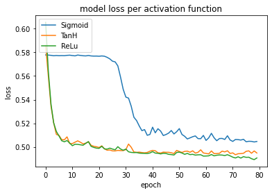
• This tutorial will introduce students to the fundamentals of the hyperparameter tunning for an artificial neural network. This tutorial will consist of the trailing of multiple hyperparameters and then evaluation using the same models configurations as the Lecture (Lecture 3). This tutorial will focus on the systematic modification of hyperparameters and the evaluation of the diagnostic plots (using loss - but this could be easily modified for accuracy as it is a classification problem) using the Census Dataset. At the end of this tutorial (the step by step examples) students will be expected to complete a Practical with additional evaluation for fairness (based on subset performance evaluation).
• Notes:
  • There is preprocessing conducted on the dataset (included in the notebook), however, this is the minimum to get the dataset to work with the ANN. This is not comprehensive and does not include any evaluation (bias/fairness).
  • We will use diagnostic plots to evaluate the effect of the hyperparameter tunning and in particular a focus on loss, where it should be noted that the module we use to plot the loss is matplotlib.pyplot, thus the axis are scaled. This can mean that significant differences may appear not significant or vice versa when comparing the loss of the training or test data.
  • Some liberties for scaffolding are presented, such as the use of Epochs first (almost as a regularization technique) while keeping the Batch size constant.
  • To provide clear examples (ie. overfitting) some additional tweaks to other hyperparameters may have been included to provide clear diagnostic plots for examples.
  • Once a reasonable capacity and depth was identified, this as as well as other hyperparameters, are locked for following examples where possible.
  • Finally, some of the cells can take some time to train, even with GPU access.
• The students will be presented with several steps for the tutorial:
  • Step 1: Some basic pre-processing for the Adult Census dataset
  • Step 2: Capacity and depth tunning (including the following examples):
    • No convergence
    • Underfitting
    • Overfitting
    • Convergence
  • Step 3: Epochs (over and under training - while not introducing it as a formal regularization technique)
  • Step 4: Activation functions (with respect to performance - training time and in some cases loss)
  • Step 5: Learning rates (including the following examples):
    • SGD Vanilla
    • SGD with learning rate decay
    • SGD with momentum
    • Adaptive learning rates:
      • RMSprop
      • Adagrad
      • Adam
• The subgoals for these five parts is to provide students with examples and experience in tunning hyperparameters and evaluating the effects using diagnostic plots.

Time: 60 minutes

Outline/time schedule

Duration (Min)	Description
5	Pre-processing the data
10	Capacity and depth tunning (under and over fitting)
10	Epochs (under and over training)
10	Batch sizes (for noise suppression)
10	Activation functions (and their effects on performance - time and accuracy)
10	Learning rates (vanilla, LR Decay, Momentum, Adaptive)
5	Recap on some staple hyperparameters (ReLu, Adam) and the tunning of others (capacity and depth).

Acknowledgements

Keith Quille (TU Dublin, Tallaght Campus) http://keithquille.com

The Human-Centered AI Masters programme was Co-Financed by the Connecting Europe Facility of the European Union Under Grant №CEF-TC-2020-1 Digital Skills 2020-EU-IA-0068.

Lesson plan on SURF

WikiWijs page